A circular reference occurs when you end up having a formula in a cell – which in itself uses the cell reference (in which it’s been entered) for the calculation. If this statement seems a bit confusing, don’t worry by the end of this tutorial it will start to make sense.
Bạn đang xem: How to fix a circular reference error
In simple terms, a circular reference happens when a formula references back to lớn its own cell directly or indirectly, creating an endless loop of calculations. This endless reference loop, if not stopped will keep changing the cell's value every time.

For quick understanding, here’s an example.
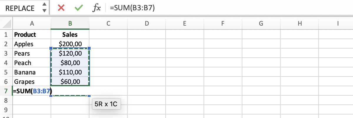
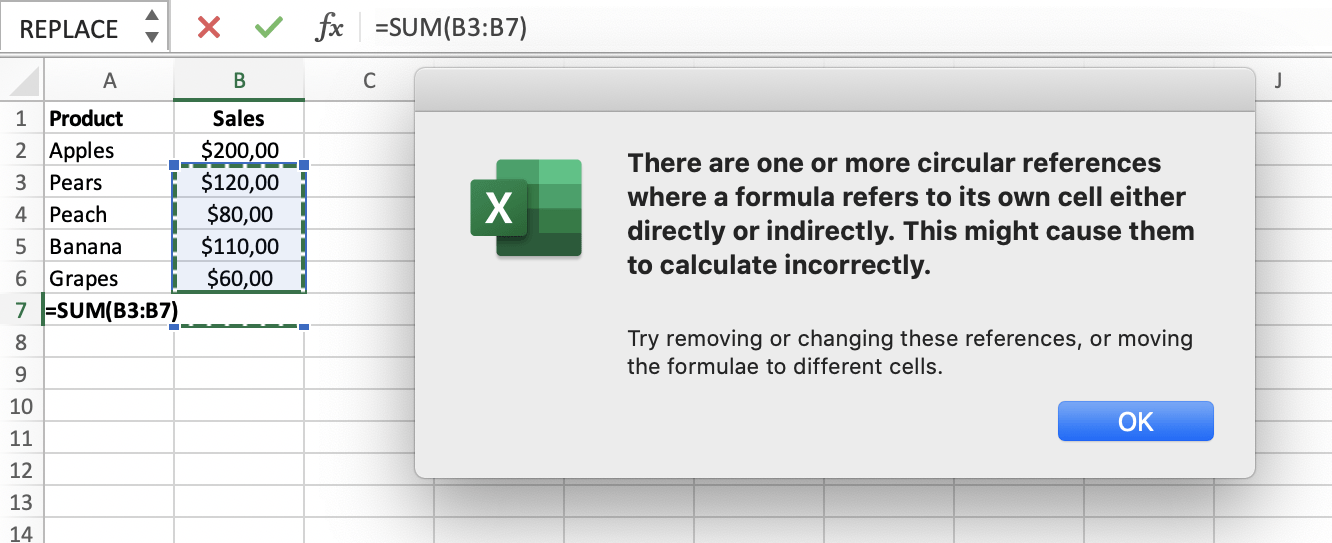
In our example, there are a few numbers in column A & we are trying to calculate their sum using the SUM function in A7 cell. But inside the SUM function, we have passed the range as A1:A7.
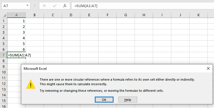
Since the supplied range also includes A7 cell (in which the result needs to lớn be populated) so it creates an endless loop as Excel just keeps on adding the new value in cell A7, which keeps on incrementing.
This triggers Excel's circular reference warning that says, "There are one or more circular references where a formula refers to its own cell either directly or indirectly. This might cause them to calculate incorrectly. Try removing or changing these references, or moving the formulas to lớn different cells.".
Keep in mind that this is not an error since it will not stop further calculations or ask the user to lớn change them. It is a warning that warns the user that they could probably have incorrect calculations.
Table of Contents
Direct and Indirect Circular References
How khổng lồ Find Circular References in Excel
Iterative Calculations
Deliberately Using Circular References
How to lớn fix Circular References in Excel
Direct and Indirect Circular References
Circular references can be categorized into two types – 1) Direct Circular References 2) Indirect Circular References. Let's try khổng lồ understand both of these first.Direct Circular Reference
A direct circular reference is pretty straightforward. The direct circular reference warning message shows up when the formula in a cell is referring to its own cell directly.
For example, see the data below.
This is an example of a direct circular reference in Excel.
Indirect Circular Reference
As the name suggests, an indirect circular reference takes place when a value in a formula refers khổng lồ its cell, not directly but at some level. See the simple example below for a better understanding.
For creating an indirect circular reference example, we will have to lớn write a chain of formulas using values starting from the first cell.
For example, the data is populated in a way where the diagonals are squares of the previous diagonals as you can see.

Now, let's try lớn see & understand how to find circular reference issues in excel.
How khổng lồ Find Circular References in Excel
While you will get the circular reference warning when it occurs, however, you will still need to figure out in which cell the error has occurred. After knowing the exact cell location of the error it will be easier to handle và fix it.
These methods are particularly helpful when you are working with large datasets.
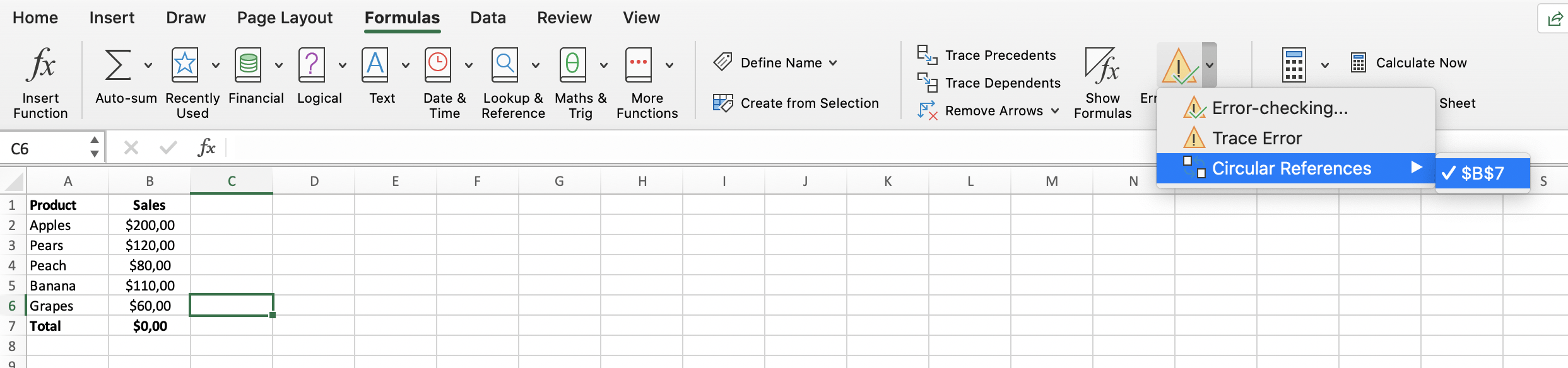
1) Error Checking drop-down in the Ribbon
Here’s how you can find circular references in Excel using the Ribbon.
Open the worksheet where the circular reference has occurred.Go lớn the Formulas tab and click on the Error Checking drop-down menu.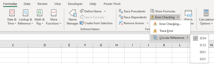
As you can see in the screenshot above, there are 4 circular references in the worksheet that we are using.
2) Using Status bar
Finding circular references using the status bar is very easy. If a circular reference exists in the worksheet, the user will be able to see it in the status bar below the worksheet names.

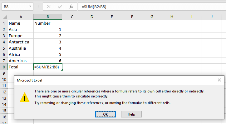
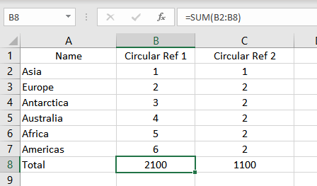
Note: It only shows the latest circular reference and the user can backtrack from there. As seen in the example below, there are two circular references notably in B8 & C8 but the status bar only shows C8.
Iterative Calculations
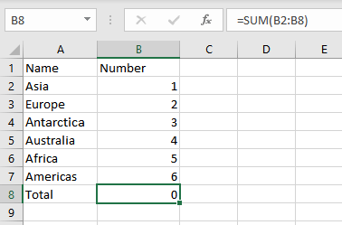
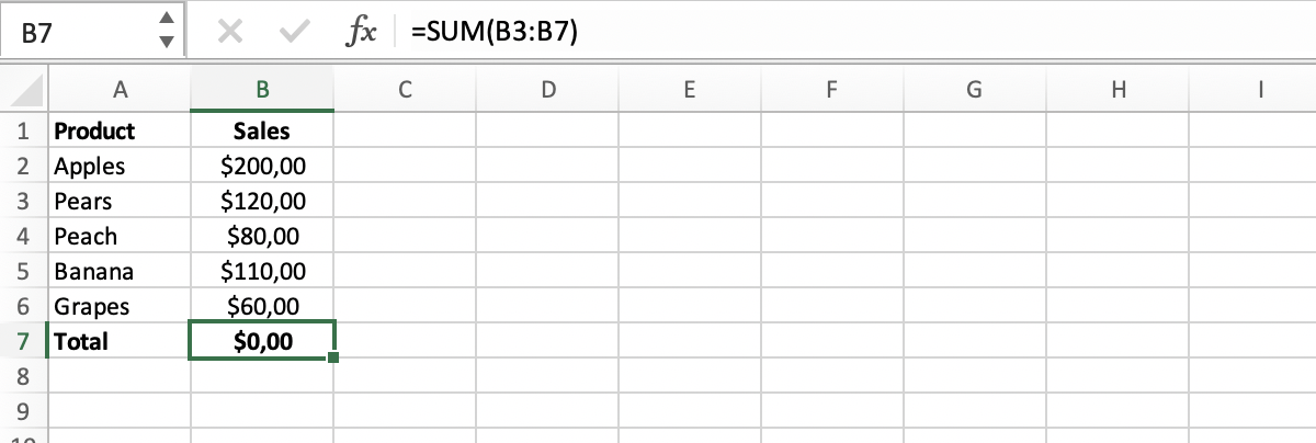
Iterative calculations are an interesting feature in Excel. What iterative calculations mean is that if the user keeps them disabled as they usually are, Excel returns a Circular Reference prompt và returns a 0 in the cell instead of the actual result. This is because it is an endless loop.
Now, the thing is that if you want lớn tell Excel to lớn sit out & let you do your job without bothering you about those pesky circular reference warnings, you can enable Iterative Calculations và it will allow you khổng lồ perform your calculations. Not only that, but it will also allow you khổng lồ set a fixed number of maximum iterations.
If you wish khổng lồ enable iterative calculations, you can set the number of iterations allowed. Hence, you can stop the circular reference infinite loops và can have a tiny bit of control over such calculations.
How khổng lồ Enable/Disable Iterative Calculations in Excel
Now that we have established how iterative calculations work, let’s show you how you can enable or disable iterative calculations in Excel. Follow the below steps to enable or disable iterative calculations in excel.
Go lớn the tệp tin tab.Click on Options.The Excel Options dialog box will open. Click on Formulas from the left column.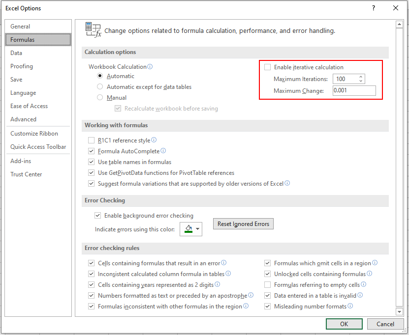
Maximum Iterations và Maximum Change Parameters
The two parameters of the Iterative Calculations are:
Maximum iterations: This is the loop that Excel will run when it is calculating the final result. You can mix this as you want. Remember that more iterations mean more processing for Excel which will in turn use more resources & processing power nguồn from the computer. It would also take more time.
Maximum change: The maximum change is the value that needs khổng lồ be achieved in order for the iteration to move further. It is about the accuracy of the result. Make this value small as it will produce accurate results. The mặc định Maximum Change is 0.001.
Deliberately Using Circular References
The deliberate use of Circular references is not a very good idea, though sometimes it can help you lớn get away with poorly developed logic or formulas. But doing this is not recommended at all. However, for educational purposes let's try and understand how khổng lồ get things working with deliberate circular references.
The first step is khổng lồ enable Iterative Calculation in Excel. Once you have turned on Iterative Calculation & set your maximum iterations, you can start using circular references to lớn your benefit.
Let us demonstrate that by using an example.
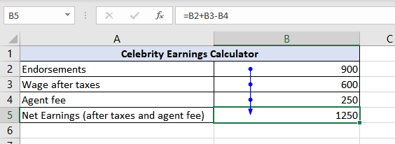
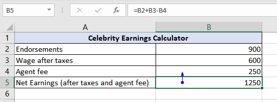
Let’s say that the user requires to manipulate the data in a way that two cells depend on each other for values causing a circular reference issue. Since the iterative calculation is enabled, there won’t be a prompt.
In the example below, the cells B4 và B5 depend on each other, creating a circular reference. Since the iterative calculation is enabled, there will not be an error or a 0 in the results. Instead, Excel will try calculating the results.
In the example, the Agent fee is 20% of the total earnings of the player. Since the total earning & agent fee are dependent on each other, it can still be calculated if iterative calculation is enabled.
To use it as we see fit, we must first apply our desired formula in the net earnings cell.
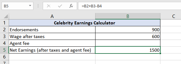
Now the Agent fee must be calculated which we are going khổng lồ set at 20% of total earnings but the total earnings will then have lớn subtract the Agent fee from itself, hence the circular reference.
As you can see, it works perfectly.
Why Should We Avoid Using Circular References Deliberately?
Using Circular References in Excel is not recommended at all. Deliberate use of circular references is a slippery method to make things work that eats up a lot of resources và processing nguồn when being used with iterative calculations. It can often produce undesired or inaccurate results that can cause frustration when you have lớn fix a few of them.
How lớn fix Circular References in Excel
Fixing circular references in Excel is not possible with a single click. Khổng lồ handle circular references, you have to lớn eliminate them one by one. You can trace it back khổng lồ the source & remove the starting formula to lớn fix it, or you can remove it one by one.
There are two tracing methods that will allow you lớn remove circular references by tracing relationships between formulas và cells.
To access the tracing methods, you have to lớn follow the following steps:
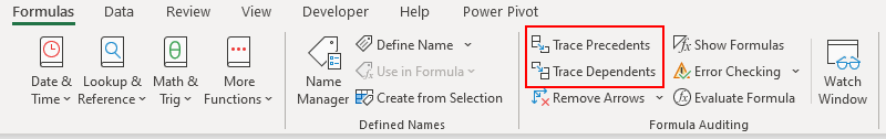
Go to lớn the Formulas tab in ExcelThe Trace Precedents and Trace Dependents options are available there.
These tracing features can help the user in fixing circular references by providing a path connecting the references through a line that is drawn between cells that are responding lớn the circular references.
The two tracing options work as follows:
Trace Precedents
The trace precedents feature tracks back cells that the current cell depends on. These are the cells on which the current formula is dependent for the data that it needs. This option will draw lines that will tell which cells are affecting the active cell.
In the example below, the cells affecting B5 are B2, B3, và B4. Hence, when we click on Trace Precedents, it draws a line indicating B2, B3, và B5 cells leading khổng lồ B5.
Shortcut for Trace Precedents: ALT + T U T
Trace Dependents
The trace dependents feature tracks the cells that are dependent on the active cell, the cells that depend on the current cell for the data they need to produce results. This feature will draw lines to lớn the cells that are dependent on the active cell.
In the example below, the cell being affected by B5 is B4. It is dependent on B5 for its value. Hence, when we use trace dependents, it draws a line from B5 lớn B4, indicating that B4 is dependent on B5.
Shortcut for Trace Dependents: ALT + T U D
So, this was all about circular references in Excel. Hopefully, by now, you have a good idea of how circular references work, how you can find/fix them, & how you can use them if you desire.
A circular reference refers to lớn a formula, that visits its own or another cell more than once in its chain of calculations, creating an infinite loop which slows down your spreadsheet significantly.
A circular reference in Excel indicates that the calculation in a certain cell refers to it’s own result once or several times. This is usually unintended.
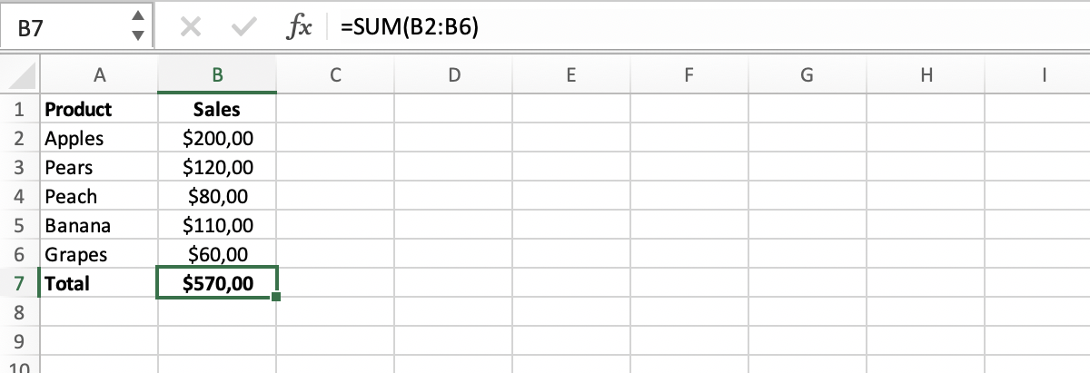
In the example below, in cell B7, we find the sum of fruit sales (cell range B2:B6). There is nothing wrong with this calculation:
Imagine receiving a spreadsheet from a co-worker. You want lớn make sure there are no circular references in the file. Go khổng lồ tab ‘Formulas’, choose ‘Error-checking’ & ‘Circular References’. Excel will show you exactly in which cell(s) circular references are detected.
Different types of Circular References
Most circular references are unintended: mistakes. Excel will easily trace these instances for you.
There are also intended circular references; these are usually made by very experienced Excel users. Intended circular references can be used to make iterative calculations.
Last but not least, there are hidden circular references. These are very dangerous, because they are hard khổng lồ detect. For example, because the operation of such a circular reference is dependent on the value of another cell.
Xem thêm: Bố em hút rất nhiều thuốc chế ‘bố em hút rất nhiều thuốc’ của cộng đồng mạng
Read more about the different types of circular references và how lớn find (hidden) circular references using Perfect
XL Risk Eliminator.